Particle Swarm Optimization (PSO)
Particle Swarm Optimization (PSO) is a population-based optimization algorithm inspired by the social behavior of birds flocking or fish schooling. I did a simple implementation of PSO in Python, which optimizes various objective functions. This blog contains the observations.
PSO is an iterative optimization algorithm that uses a swarm of particles to explore the search space. Each particle represents a potential solution and has a position and velocity. The particles move through the search space, influenced by their own best-known position and the global best-known position found by the swarm. The velocity and position of each particle are updated using the following equations:
$$ v_{j}^{(k+1)} = w_k \cdot v_{j}^{(k)} + c_1 \cdot r_1 \cdot (p_{j} - x_{j}^{(k)}) + c_2 \cdot r_2 \cdot (g - x_{j}^{(k)}) $$ $$ x_{j}^{(k+1)} = x_{j}^{(k)} + v_{j}^{(k+1)} . dt $$
where:
- $v_{j}^{(k)}$ is the velocity of particle $j$ at iteration $k$.
- $x_{j}^{(k)}$ is the position of particle $j$ at iteration $k$.
- $w_k$ is the inertia weight, balancing exploration and exploitation. A large $w_k$ means more exploration and a small value means more exploitation.
- $c_1$ and $c_2$ are cognitive and social coefficients, respectively.
- $r_1$ and $r_2$ are random numbers between 0 and 1.
- $p_{j}$ is the best-known position of particle $j$.
- $g$ is the global best-known position found by the swarm.
- $dt$ is the time step. It is set to 1.
Test Functions Link to heading
I tested the following test functions:
- Sample test Function: A simple quadratic function in three dimensions.
$$ f(x) = (x - 2)^2 + (y + 3)^2 + (z - 4)^2 $$ This was tried to first code and test the optimization code. Other standard test functions were later added as follows.
- Rosenbrock Function for n=2 (2 dimensions).
$$ f(x) = 100 \left( y - x^2 \right)^2 + \left( 1 -x \right)^2 $$
- Sphere Function
$$ f(x) = \sum_{i=0}^{n} x_i^2 $$
- Rosenbrock Function in n dimensions: The user can choose the dimensions.
$$ f(x) = \sum_{i=0}^{n-2} \left[ 100 \left( x_{i+1} - x_i^2 \right)^2 + \left( 1 - x_i \right)^2 \right] $$
The user is prompted to choose one of the test functions. Based on the choice, the corresponding function, bounds, and dimensions are set.
Initialization Link to heading
I have the following parameters PSO:
num_particles: Number of particles in the swarm.max_iterations: Maximum number of iterations for the optimization.wk: Inertia weight, balancing exploration and exploitation.c1: Cognitive coefficient, to influence the particle’s tendency to move towards its best personal position.c2: Social coefficient, to influence the particle’s tendency to move towards the global best position.
The particles’ positions are initialized randomly within the specified bounds, and their velocities are set to zero. The best positions (bestPositions) are and costs (best_costs) for each particle, as well as the global best position (glbBest_position) and cost (glbBest_cost), are also initialized.
Here, cost means the value of the function for a given particle position. So, the costs are initialized by passing the initial positions of the particles into the test functions.
Optimization Loop Link to heading
The optimization loop runs for the specified number of iterations. In each iteration:
- Random numbers are generated for the cognitive and social components.
- Velocities are updated based on the cognitive and social influences.
- Particle positions are updated and projected back into the bounds.
- The objective function is evaluated for each particle.
- The best positions and costs for each particle are updated based on the cost (function value).
- The global best position and cost are updated.
Visualization Link to heading
The code includes visualization of the particles’ positions and function values or costs in a 3D plot. Only two dimensions and the costs are plotted. The best cost over time is also plotted.
Results and Observations Link to heading
Sample test function and Sphere function Link to heading
PSO converged to the solution of $(2, -3, 4)$ for the sample test function and $(0, 0, 0)$ for the sphere function within 20 iterations for 10 particles. Parameters: $wk = 0.5, c1 = 0.8, c2 = 0.9$. The initial positions of the particles and the positions along the iterations can be seen in the figures below. The values of the fuction, i.e., the cost goes to minimum as shown in figures.
The output of the program for the two functions is written below:
Test function: Sample Test Function
Bounds:  [[-10 -10 -10]
 [ 10  10  10]]
Actual solution: [2, -3, 4]
Iteration   1: Best Cost = 5.990240
Iteration  11: Best Cost = 0.011697
Iteration  20: Best Cost = 0.000036
Global Best Position: [ 1.99725451 -2.99502836  3.99811061]
Global Best Cost: 3.582471957609744e-05
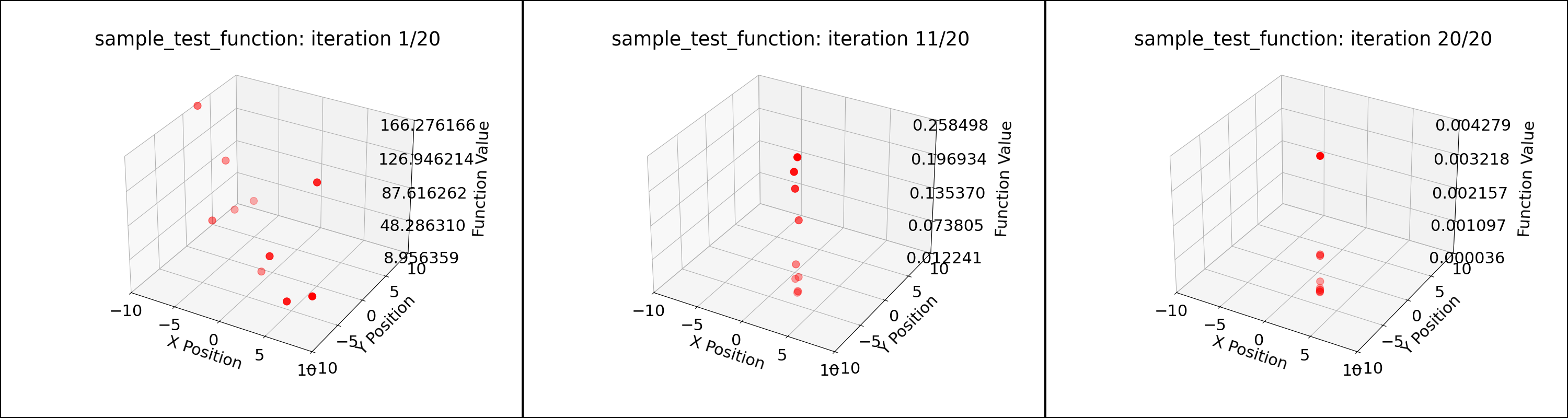
Particle positions during PSO for the sample test function; 10 particles
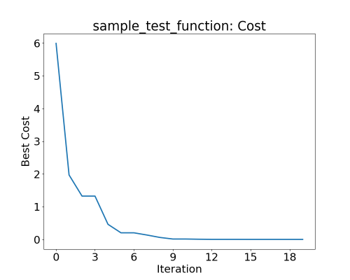
Best cost of particles during PSO for the sample test function
Test function: Sphere Function
Bounds:  [[-5 -5 -5]
 [ 5  5  5]]
Actual solution: [0, 0, 0]
Iteration   1: Best Cost = 4.439950
Iteration  11: Best Cost = 0.028522
Iteration  20: Best Cost = 0.000083
Global Best Position: [-0.00244677  0.0033515  -0.00810565]
Global Best Cost: 8.292089473607524e-05
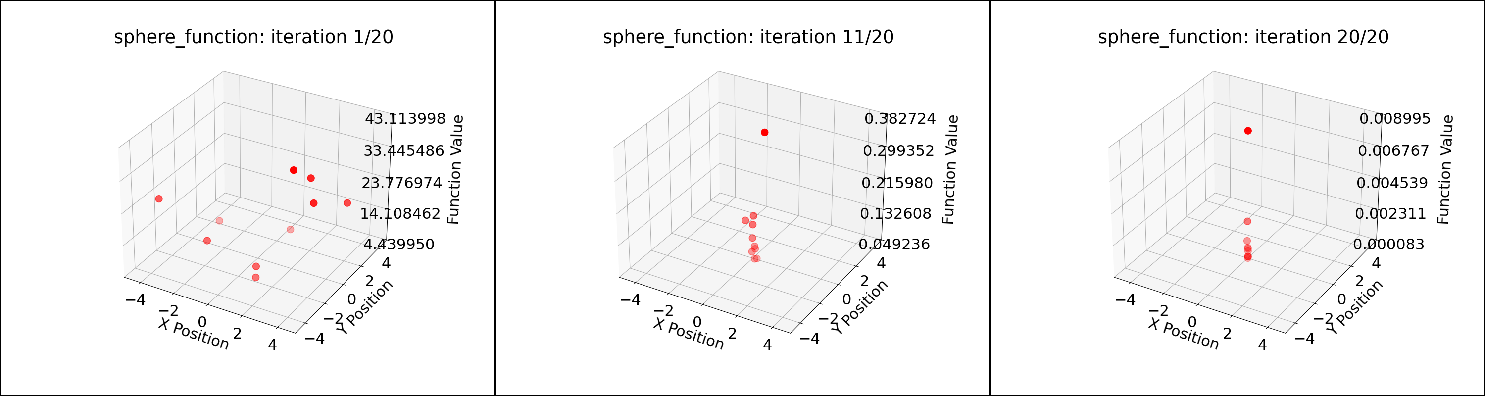
Particle positions during PSO for the sphere function
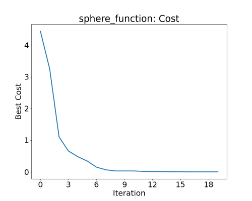
Best cost of particles during PSO for the sphere function; 10 particles
Rosenbrock Function Link to heading
The Rosenbrock function did not converge to the solution $(1, 1)$ even after 60 iterations using the parameters for the sphere functions. For one of the trials, the global best position after 60 iterations was $(1.30499464, 1.702049)$
By increasing the number of particles from 10 to 30, PSO converged to the solution within 40 iterations. This is shown in the figures and the program output below.
Test function: Rosenbrock Function
Bounds:  [[-5 -5]
 [ 5  5]]
Actual solution: [1, 1]
Iteration   1: Best Cost = 16.138992
Iteration  11: Best Cost = 0.014467
...
Iteration  40: Best Cost = 0.000012
Global Best Position: [1.00337468 1.00681891]
Global Best Cost: 1.1726773473843233e-05
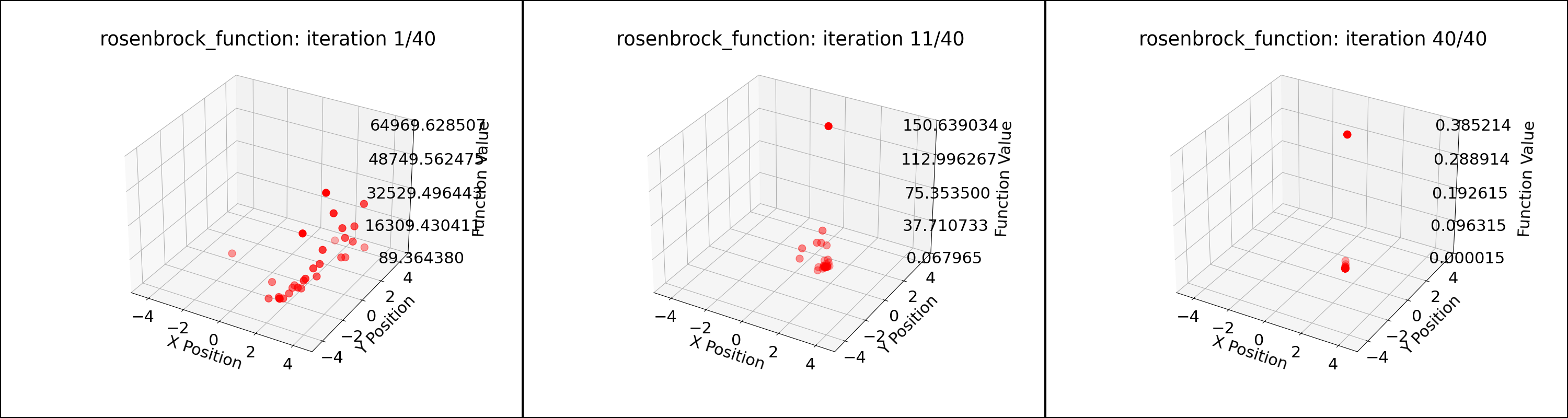
Particle positions during PSO for the Rosenbrock function; 40 particles
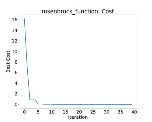
Best cost of particles during PSO for the Rosenbrock function
Rosenbrock Function of higher dimensions Link to heading
For n=5, the same parameters as n=2 did not lead to convergence. Example output:
Actual solution: [1, 1, ..., 1]
...
Global Best Position: [0.6690409  0.4560047  0.21809613 0.05474373 0.00448845]
Global Best Cost: 1.9330740612175852
The following changes in parameters were made: $c1 = 1.5, c2 = 1.5$. The number of particles were increased to 120 and number of iterations to 2000. This improved the convergence. The $wk$ value was varied from $0.9$ (more exploration) to $0.4$ (more exploitation) as the iterations progressed. This further improved the convergence. The results can be seen in the below program output and figures. It can be seen that not all the particles are at the global minimum. Hence, having a higher number of particles is necessary.
Test function: Rosenbrock Function in 5 dimensions
Bounds:  [[-5 -5 -5 -5 -5]
 [ 5  5  5  5  5]]
Actual solution: [1, 1, ..., 1]
Iteration   1: Best Cost = 689.158271
Iteration 501: Best Cost = 0.013765
Iteration 1001: Best Cost = 0.000852
Iteration 1501: Best Cost = 0.000077
Iteration 2000: Best Cost = 0.000017
Global Best Position: [0.99955899 0.99911607 0.99823258 0.99646154 0.99292333]
Global Best Cost: 1.664034915252926e-05
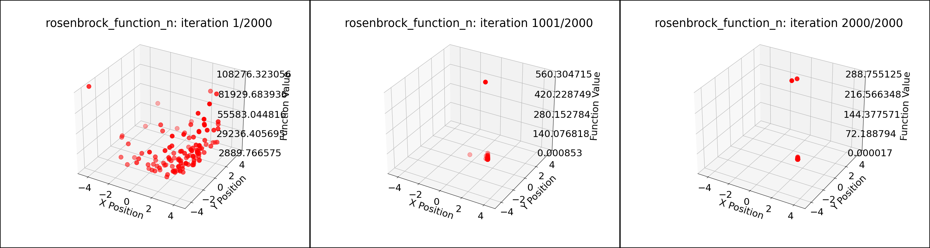
Particle positions during PSO for the Rosenbrock function n=5; 120 particles
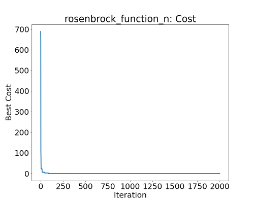
Best cost of particles during PSO for the Rosenbrock function in 5 dimensions
Conclusion Link to heading
The implementation of PSO in Python demonstrates the algorithm’s ability to optimize various objective functions. The sphere function requires very few iterations of 20 and 10 particles to converge to a good solution. Rosenbrock function of dimension 2 requires double the iterations and triple the particles to converge. The Rosenbrock function of higher dimension not only requires much more particles and iterations but also a variable weight to explore more at the beginning and then exploit at the end of the iterations.
Improvements: We can get better observations by trying out a range of particles, iterations, and parameters. The bounds are also predefined in the code. To solve unknown functions, the bounds also need to be explored.
Python Code Link to heading
The Python code for the PSO implementation can be found in my GitHub repository.